1The water cycle
1.1Hydrological framework: Water fluxes in the soil - plant - atmosphere continuum
Ancien text a revoir ou supprimer compte tenu de la section rajoute au tout debut (conceptual framework)
The transpiration sink in equation 5.1 describes the interplay between the transpiration flux, , the soil moisture profile, and the root density profile, which is assumed to decrease exponentially with depth, with a decay factor depending on the PFT (Table Y):
Bare soil evaporation is a parallel flux to transpiration, which originates from the entire bare soil column, and from the bare soil fraction of the other soil columns. It is described based on a supply/demand approach:
where the demand is defined by , the potential evaporation reduced following Milly (1992), and the supply by , the maximum amount of water that can be extracted from the soil given the moisture profile (thus at the soil column scale). To prevent from mass conservation violation, is estimated by dummy integrations of equation 5.1 at the end of each time step, in which two boundary conditions are successively tested: firstly a flux condition favoring the demand (); then, if the previous case leads to any node with , a Dirichlet condition ( at the top node), which strongly limits . The resulting water stress factor (, equation 3.y) will control and the surface energy budget of the next time step. If the total moisture in the top 4 soil layers (assumed to be representative of the litter) is below the wilting point, this stress factor is arbitrarily reduced by a factor 2. Eventually, can proceed at the potential rate of Milly (1992), unless water becomes limiting, i.e. if upward diffusion to the top soil layer cannot provide enough water to sustain the demanded rate.
[AD] This needs to be made consistent with sections 3.1 and 3.4. The case of the bare soil “PFT” needs to be checked, especially for the root decay factor (=5 in the default values). Check if a weighting by the vegetation fractions fvj is required somewhere for transpiration (idem for 1- fvj and bare soil evaporation).
A separate soil water budget is performed in each soil column within a grid-cell. At each time step, the liquid water input to a soil column comprises through-fall and snowmelt, averaged over the contributing PFTs. Given the spatial average of bare soil evaporation and transpiration over the contributing PFTs, the soil hydrology scheme integrates the soil moisture variations over the time step, calculates the output water fluxes (surface runoff and drainage), and diagnoses the water stress factors to calculate the forthcoming evaporative fluxes and feed the STOMATE module (crossref). As detailed in Rosnay (2002) and Campoy et al. (2013), soil water redistribution in the soil implies 1-D vertical water fluxes,
In all cases, and are linearized in the variation range of (between the residual and saturated values, and ), by means of 50 piecewise functions, respectively constant and linear in (details in section 1.1.4) This allows a first-order linearization of Equation CITE EQUATION, which can thus be solved by a tridiagonal matrix algorithm. The prognostic variables are the volumetric moisture contents of each node within each soil column. Diagnostic soil moisture layers are also defined, with limits equidistant between two consecutive nodes, so that each layer holds one node. The moisture content of the layers ( in mm) is then diagnosed assuming a linear profile between two consecutive nodes.
1.2OK: Canopy interception and througfall
As described in Section 1.6.3, the canopy interception flux is calculated for each PFT. It is derived from potential evapotranspiration, moderated by a resistance factor specific to the interception process. This resistance factor incorporates both the aerodynamic and vegetation structural resistances, and is further weighted by the fraction of vegetation that holds intercepted water , defined as:
Where is the fraction of vegetation covered by the PFT, is the amount of water intercepted by that PFT per unit of surface (kg m), and is the maximum amount of water that can be intercepted by that PFT per unit of surface (kg m).
The maximum amount of water intercepted is controlled by the leaf area index (m m) and an arbitrary constant , which transforms into the size of the interception reservoir (unitless), following:
The vegetation canopy is assumed to form a continuous layer, with gaps represented by a supplementary bare soil fraction. For each PFT, the intercepted water storage is first updated by subtracting the interception loss flux over the timestep (Eq. CITE EQUATION Section 1.6.3):
This term represents the loss of water from the interception reservoir due to wet-canopy evaporation. In principle, rainfall first wets the canopy, and only the excess drips to the soil from the intercepted reservoir. In that idealized case, the increase of canopy water storage from a rainfall input would be proportional to the vegetation cover fraction of the PFT:
In reality, however, not all intercepted water remains on the canopy: some evaporates back to the atmosphere (Eq. 151), and some drips to the soil. These processes occur on short time scales (minutes), while the model time step averages precipitation over longer intervals. As a result, the model cannot explicitly resolve the rapid balance between interception, dripping, and evaporation. To account for this limitation, ORCHIDEE prescribes a throughfall fraction that forces a fraction of rainfall to reach the soil directly. The increase in canopy water storage over the model timestep is then reduced accordingly:
As mentioned previously, canopy storage is limited by a maximum capacity . When the reservoir exceeds this maximum amount, the canopy water storage is capped and the excess drips into the soil :
The input of water to the ground for each PFT , therefore includes three contributions: direct throughfall, drip from canopy reservoir overflow, and rainfall onto the unoccupied fraction of the PFT:
Where is the maximum fraction of the PFT (unitless).
The volumetric ratio is then a proxy for the actual fraction of the vegetation surface covered with water.
In addition to rainfall, the canopy can also intercept dew (provided it is not freezing). Dew is assumed to behave differently from rainwater: intercepted dew never drips to the soil but always evaporates back to the atmosphere. The fraction of dew that can be intercepted by leaves (unitless), is expressed as a 5-degree polynomial function of CITATION:
This parametrization is only applied for vegetated PFTs with , otherwise is set to 1.
1.3OK: Water status of plants and water transport inside the vegetation
The multi-layer soil hydrology scheme presented section 1.7 is partly driven by the vegetation transpiration. This amount of water transpired by the different PFTs (and thus extracted from each soil tiles) is controlled by the rate of aperture of the stomata. This rate of aperture, hereinafter mentioned as stomatal conductance, is regulated by several environmental and physiological factors such as the sensitivity to vapour pressure deficit, leaf sugar concentration and plant hydraulics Damour et al., 2010. This latter stomatal conductance driver, plant hydraulics (and their link to soil moisture), is an essential process to take into account to regulate stomatal aperture and leaves-atmosphere exchanges. It is usually modeled either through an empirical function directly applied to the stomatal conductance formulation Mencuccini et al., 2019Fatichi et al., 2016 or a full representation of the water flow inside the soil-plant-atmosphere continuum which enables the representation of the plant water potentials and a direct control of the stomatal conductance by the leaf water potentials Kennedy et al., 2019Kauwe et al., 2020. In the ORCHIDEE-trunk, both formulations are proposed: i) the historical empirical control of stomatal conductance by soil moisture, described in section 1.3.1; or ii) a plant hydraulics control of stomatal conductance following the implementation of Alléon et al. (submitted), described in section 1.3.3.
1.3.1OK: Empirical dependence
In its standard configuration, the stomatal conductance formulation follows Yin & Struik (2009) (more details on the photosynthesis resolution in section 1.2). In this model, stomatal conductance is directly driven by two empirical functions which describe respectively the sensitivity of the stomata to leaf-to-air vapour pressure deficit (approximated here by the air vapour pressure deficit (VPD)) and the sensitivity to soil moisture deficit. For each LAI layer , the stomatal conductance then follows:
where and represent the inter-cellular partial pressure and the compensation point in absence of day respiration ( mol.mol), and represent the assimilation rate and the day respiration ( mol[CO].m.s), is the residual stomatal conductance (mol[CO].m.s). Finally, G and G represent the sensitivities to VPD and soil moisture deficit. They follow respectively:
Where (unitless, set to 0.85) and (which equals 0.14 kPa) drives the sensitivity to , corresponds to the fraction of root located in soil layer , with , , represent respectively the soil water contents (kg/m): in layer , at field capacity, and at the wilting point. is the threshold water content under which stomatal conductance sensitivity starts to decrease linearly and which, with (unitless, set to 0.8), puts the start of tranpiration stress at on the segment from to . is the sum of the soil moisture stress across layers, weighted by the root profile.
A non-linear alternative soil water stress can be calculated with the following equation:
ADDED material from Agnes paper
The transpiration sink in Eq. 159 describes the interplay between the transpiration flux, , the soil moisture profile, and the root density profile.
The resulting shapes of the transpiration stress factor are illustrated in Figure 6 for the various soil textures considered in ORCHIDEE.

Figure 6:Variations of the transpiration stress factor as a function of mean volumeric water content in the soil layer (VWC), assuming a uniform VWC profile for simplicity. why is this assumption needed
Importantly, all above variables are actually defined at the PFT level, but the index of the PFT was omitted for simplicity. The aggregation at the grid-cell scale is additive, for both the transpiration flux and the total sink term , which correspond to the same quantity by construction:
Eventually, in each PFT, the water stress factor is involved in two ways:
its value from the previous time step defines the root sink term thus the water budget of the current time step;
once updated at the end of the current time step, based on the corresponding soil moisture, it is used at the beginning of the following time step to calculate the stress function controlling the transpiration of the PFT thus the surface energy budget of the following time step.
1.3.2Semi-empirical dependence
Describe the Meridja function for humrel
1.3.3OK: Plant hydraulics dependence
ORCHIDEE-trunk now embarks a stomatal conductance dependence on leaf water potential. In this configuration, the photosynthesis model of Yin & Struik (2009) is kept but the stomatal conductance formulation is revised and follows Tuzet et al. (2003):
Where (unitless) represents the sensitivity of stomata to a decrease in leaf water potential ( in MPa):
This sigmoïdal function is driven by two PFT parameters: (in MPa), the reference water potential which engenders approximately a 50 % stomatal closure and (in MPa), the sensitivity to leaf water potential decrease.
The computation of relies on the representation of water transport from the soil-root interface towards the stomata. In this representation, two water storage pools (for the trunk and the leaves) are defined by capacitances and a set of fixed resistances is defined to model the water flow between each node (i.e root surfaces, trunk-root interface, trunk-trunk storage interface, trunk storage, trunk-leaf storage interface, leaf storage, stomatal cavities) via Ohm’s and Kirchoff’s current laws.

Figure 7:check whether the same symbols are used in the text and the figure. Adjust the figure to the text. Hydraulic Architecture resistance and capacitance network. For the resistances:(1) Mesophyll resistance (); (2) Trunk to leaf xylem resistance (); (3) Root to trunk resistance (); (4) Leaf storage resistance (); (5) Trunk storage resistance (); (6) Upper root system resistance (); (7) Lower root system resistance ().
Water storage pools
Each water storage pool is defined as in Tuzet et al. (2017) through capacitances (, in m.MPa with X representing either leaf or trunk storage pools) defined according to the storage pool water potential () by the following equation:
With,
Where, (m) is the maximum volume that can be stored in the pool (arbitrarily defined as 80 % of the biomass of carbon of the leaves and the sapwood as described in section 1.4.4), (m) is the residual volume of water of the pool (arbitrarily defined as 40 % of after personal communication with A. Tuzet), (MPa) is, according to Tuzet et al. (2017) a parameter depending on the morphological adaptation in different species and on environmental conditions experienced during growth and (MPa) is a reference water potential.
The dynamics of each storage pool rely on a differential equation (Eq. 165) which links the storage compartment water potential () to the flux between the trunk-storage compartment interface and node above (, in m.s), to the resistances above and below the storage compartment ( and , in MPa.s.m) and to the storage compartment resistance (, in MPa.s.m).
Both storage pool associated differential equations are solved through a predictor-corrector scheme (a two-steps resolution where the state variable at time step is firstly predicted with a classical explicit resolution and then corrected by a second calculation involving the prediction). This resolution permits to avoid instabilities when calculating the new value of the storage water potential. In this resolution, the predictor term is calculated and used as follows:
Where, corresponds to the right-hand side of Eq. 165.
This predictor-corrector scheme enables to approximate the value of the storage pool water potential at the end of the time step which, along with the value at the beginning of the time step, leads to the calculation of the water fluxes coming from or inside the storage pool.
Water absorption by roots
At the soil-root interface, the water absorption by roots is computed in two soil horizons (averaged from the multi-layer soil hydrology scheme presented in section 1.8). It can be represented by two different approaches.
In the simpler approach, a dynamic resistance is applied at the soil root interface. Its formulation (Eq. 168 for a soil layer ) follows the representation implemented by Bonan et al. (2014) (Section A4.3, Equations A23 to A25).
Where, is the total root length per unit volume of soil in the soil horizon (m.m - calculated according to root biomass), is the soil horizon height (in m), is the mean fine roots radius (which equals 0.5 mm) and is the hydraulic conductivity in layer (in mm.day).
In this framework, the soil horizon water potential and hydraulic conductivity are calculated following either Genuchten (1980) formulation or Campbell (1986) in order to avoid the numerical instabilities which can appear when the soil water content is close to the residual soil water content.
In the more complex framework, the water absorption by roots is represented following Tuzet et al. (2003). In this mechanistic representation, the volume of soil in the horizon is considered cylindrically distributed around a fictive root of length . In this cylinder of soil, Richard’s equation (Eq. 169) is solved radially which enables to compute the gradient of moisture content near the root.
where (mm.day) is the soil diffusivity and , the distance from the root axis. Richard’s equation is solved at a half hourly time step for nodes along the radial axis. At the soil-root interface (), the absorbed water flux ( or , in m.s, respectively for the upper and lower soil horizons) is applied as a boundary condition. The radial resolution of Richards’ equation is performed using the same resolution framework as the vertical water diffusion presented before (see Section 1.7). This resolution enables the calculation of the water potentials at the root surfaces ( and ), by considering a continuity between the soil water potential at the node and the root surface.
Numerical resolution
During unstressed periods, the resolution of the hydraulic architecture is purely explicit. At the beginning of the time step, photosynthesis (section 1.2) is solved and is the first calculated variable, using Eq. 161 and the leaf water potential from the previous time step. Then, the resolution of the energy budget (sections 1.1 & 1.8) enables the calculation of the transpiration flux, using . The different water fluxes within the hydraulic system are computed from the top to the bottom imposing flux as a boundary condition at the leaf level. The flux between each storage pool and the nearest node ( or ) is assessed following the predictor-corrector scheme described in the previous section. Using Kirchhoff’s current law and the storage water fluxes, all water fluxes can be determined down to , the flux between the trunk and the trunk-root interface, above the two root horizons. At this interface, the two fluxes of water uptake by roots, and , are assessed from and the root water potentials of the previous time step with Eq. 170.
Based on the two root water fluxes, water absorption by roots is solved. The water contents in the two soil layers are updated as well as the resulting root water potentials and . The other water potentials of the hydraulic system are then updated, from the bottom to the top, using the previously calculated fluxes and the water potential of the compartment down the flux. Thus, the updated water potential at a given level () is expressed as:
Where is the water potential at the level down the flux; and and are the flux and the resistance between the two levels, respectively.
During drought periods, the non linearity of the stomatal conductance formulation and the strong coupling between stomatal conductance, transpiration and leaf water potential can introduce strong feedbacks between the variables, further leading to numerical instabilities which would justify the use of an iterative resolution scheme (Alléon et al. (submitted), Yang et al. (2019)Sabot et al. (2022)). In ORCHIDEE-trunk, this drawback has been partly solved by implementing an adapted resolution scheme.
A first resolution of the hydraulic architecture model is performed using the explicit framework presented previously. This first calculation is purely diagnostic and enables the calculation of the variables at the current time step. A second resolution of the hydraulic architecture model is then launched. The objective of this second calculation is to approximate the value of the leaf water potential at the next time step in order to avoid a resulting stomatal conductance too far from reality at the next time step. To do this, an approximation of the transpiration flux at the next time step is performed. The transpiration equation can be summarized as:
where is the air density (kg.m), is the time step length, is the difference of humidity between the surface and the atmosphere (kg.kg), is the aerodynamic resistance (m.s) and is the stomatal resistance (m.s). This equation can be simplified to:
The transpiration at time step and at time step can be expressed as:
The objective here is to estimate from . Looking at the components of the transpiration:
and represent the evolution of over the day;
and represent the evolution of the aerodynamic resistance;
and represent the evolution of the components of that are not directly linked to .
The following assumptions are made:
= ;
= ;
= ;
can be estimated by a sinusoidal function centered on solar noon.
The assumption is, hence, that in the absence of water stress, transpiration and stomatal conductance will follow a sinusoidal function centered on the solar noon, starting at sunrise and ending at sunset. Following this assumption, can be expressed as the ratio between the values of the sinusoidal function at time step and . The amplitude of the sine function cancels out in the ratio.
Consequently, the ratio between and can be estimated as:
This ratio, multiplied by , permits to have a prediction of only with variables from the previous time step. This approximation enables the second solving of the hydraulic architecture and the estimation of the leaf water potential at the next time step. As the transpiration estimation is relying on the leaf water potential value at the same time step, several iterations are performed in order to make the resolution converge towards a unique leaf water potential value which will be sent to the photosynthesis module at the next time step. One can note that the scheme can be improved by improving the transpiration flux estimation.
1.4OK: Snow and land ice
The multi-layer snow scheme described and evaluated in Wang et al. (2013) is based on the ISBA-ES model (Boone & Etchevers (2001)) and has been implemented on the vegetated/biological fraction of the ORCHIDEE grid cell. Its extension to glaciers has been validated over Greenland ice-sheet (Charbit et al. (2024)) and replace the old single-layer scheme described in Chalita and Letreut, 1994. This multi-layer scheme is used to describe the hydro-thermal processes within the snowpack and solve the mass and energy balance equations.
To describe the snowpack evolution, a number of three layers was chosen, for which three prognostic variables (i.e., snow heat content, density and thickness) are calculated. Temperature and liquid water content are diagnosed at each time step and for each layer. The total snow mass and its mean density is then used to derive a snow cover fraction that enters the calculation of the surface albedo and roughness of each grid cell that contains snow, to account for the high albedo and smoothing impacts of snow Wang et al. (2013).
The multi-layer snow scheme describes the energy and mass transfers between the snowpack and the atmosphere and the main internal processes at play such as snow settling, water percolation and refreezing. The calculations are done in the following way: at each time-step, the surface flux entering the top snow layer is computed from the surface energy balance equation. Snowfall updates the thickness, density, heat content, temperature and water content of the snow layers. Compaction is then modeled, modifying layer thicknesses, densities and heat content (equations (11)-(12) in Wang et al. (2013)). Temperature is then updated, from top to bottom, taking into account the new surface temperature and the integration coefficients for the snow numerical scheme, similarly to the soil temperature scheme (ref Hourdin yyyy ?) to stick with the implicit scheme. Snowmelt is then calculated, followed by liquid water transfers and possible refreezing, energy transfers during these phase changes are accounted to update temperature, layer thickness, density and liquid water content. Sublimation is then calculated followed by snow aging, snow cover fraction and finally the surface albedo as presented in section ??
1.4.1OK: Snow energy balance
The surface flux entering the top snow layer is computed from the surface energy balance equation in the same way as for soil. At the surface of the snow, the energy budget equation is:
Where is the soil heat flux due to heat conduction process; is the energy released by rainfall (see Eq. (14) in Boone & Etchevers (2001)). , , and are the net radiation, sensible heat and latent heat flux respectively (); is the surface heat capacity of soil per unit area () and is computed as the sum of heat capacities for snow-covered and snow-free surfaces weighted by their respective grid cell fraction.
The heat conduction flux into the soil is used to compute the surface temperature of the grid cell at the next time step and provides the limit condition of the surface temperature at the snow-atmosphere interface for the calculation of the snow temperature profile.
Above snow-covered surfaces, when is above the freezing temperature (273.15 K), the energy excess is first used to bring the snow temperature to . A surface energy flux associated with the freezing temperature can be computed using a similar formulation to Eq. 177. The difference between and is converted in an additional temperature expressed as:
If is greater than , the energy excess is used for melting snow, and is further set to for energy conservation. If the new value is greater than the total heat content of the snowpack, snow is entirely melted and the excess energy is transferred to the underlying soil. The energy released by snowfall is accounted for in the snowpack scheme to update the snow heat content of the snowpack after a snowfall event.
The sensible and latent heat fluxes computed for each grid cell are given respectively by:
where is the air density, and are the surface and the 2 m atmospheric temperatures, and are the air specific humidity at 2 m and the saturated specific humidity at the surface, is the latent heat of sublimation (2.8345 106 J kg-1), U is the wind speed at 10 m and is the drag coefficient computed as a function of the ice roughness length (), following the Monin-Obukhov turbulence similarity theory (Monin & Obukhov (1954)) and the parameterizations of the eddy fluxes proposed by Louis (1979).
1.4.2OK: Snow layering
In the initial version of ORCHIDEE explicit snow, the snow was distributed over 3 layers, with the first layer limited to a depth of 5cm and the second to 50cm. This vertical discretisation described in Wang et al. (2013) is still available but we now use a new discretisation with 12 layers. With this new version, the maximum thickness of the first 3 layers is respectively 1, 5 and 15cm, which limits the bias on the surface temperature. An application to the Greenland ice sheet Charbit et al. (2024) has shown that this new 12 layers scheme provides a better simulation of snow evolution than the previous 3 layers model. The definition of snow layer thickness followed the layering scheme proposed by Decharme et al. (2016) for ISBA-ES: In theses equations, identifies the snow layer and D the snow layer thickness
where the constants are the maximum snow depth for a layer with , , , , , , , , . For very thin snowpack (less than 0.1 m), each layer has the same thickness and when the snow depth is above 0.2 m, the first and last layers reach their constant values of 0.01 and 0.02 m. The layer thickness are updated if one of the first two layers or the bottom layer become too thin or too thick:
For example, if the thickness of the top layer becomes lower than 0.005 m or greater than 0.015 m, all the layer thicknesses are recalculated with Eq. 181 and the snow mass and heat content are redistributed accordingly.
1.4.3Ok: Snow compaction
When a snowfall occurs, the snow depth increases, but the depth decreases with compaction. This is why compaction is a particularly important process for the evolution of the density and depth of snow in each layer. Two processes are responsible for compaction: the weight of the overlying snow layers and the metamorphism of the snow. These two processes are taken into account in the following equation derived from Anderson (1976):
The first term of the right-hand side of equation 183 represents the compaction due to snow load with (Pa) being the pressure of the overlying snow and (Pa.s) the snow viscosity. The viscosity is an exponential function of snow temperature and density (equation 184, Mallor (1964) and Kojima (1967)):
with =3.7 10 Pa s, =8.1 10 K and =1.8 10 m kg.
The second term of the right-hand side of equation 183 represents the effect of metamorphism:
with a = 2.8 10 s, b = 4.2 10 K, c = 460 kg m and = 150 kg m. In the model, the density cannot exceed a threshold fixed at 750 kg m. Compaction does not affect the total mass and the heat content of the snowpack but changes the layer thicknesses, this is the reason why the snow heat within the layers must therefore be updated.
1.4.3.1OK: Heat content
For processes linked to phase change, we use the equation of the heat content of snow (equation 186). This allows to determine whether the snow is cold (dry) or warm (wet). The heat content of each snow layer is computed using the following equation:
where L is the latent heat of fusion and T the triple-point temperature for water. H is the total heat content, c the snow heat capacity (J.m-2 K-1) and W liquid content for the i layer. According to equation 186, heat content is used to diagnose the snow temperature assuming that there is no liquid water in the snow layer. If the calculated snow temperature exceeds the freezing point, snow temperature is set to T and the liquid water content is diagnosed from equation 186.
1.4.3.2OK: Melt and refreezing
When melting occurs at the surface, the liquid water remains in the first layer if the maximum liquid water threshold has not been exceeded. When the amount of liquid water exceeds this threshold, the water percolates into the lower layer. The water can then either refreeze or be added to the existing liquid water, depending on the temperature of the snow layer. The maximum liquid water holding capacity is taken as a function of the snow layer density following Anderson (1976).
with =0.03, =0.10 and =200 kg m.
When the liquid water reaches the bottom layer and exceeds the total liquid water content, it is then considered as runoff.
1.4.3.3OK: Heat conduction
The heat conduction from the surface to the bottom of the snowpack is described by a vertical diffusion equation relating the temporal evolution of the snow temperature in the snowpack at a depth z and the divergence of the snow heat flux F and is solved using an implicit numerical scheme.
with the snow thermal conductivity (W m K). At the snow-atmosphere interface, the boundary condition is given by the energy balance equation 177.
Along with the thermal gradient, a water vapor diffusive flux takes place from the warmer to the colder parts of the snowpack and sublimation or condensation may occur in the pore spaces depending on the water vapor saturation pressure. This process is particularly significant in the Arctic because of strong temperature gradients between soils and atmosphere and is in great part responsible for snow metamorphism. While it is explicitly accounted for in detailed snow models, in Explicit Snow, the effect of water vapor diffusion and phase changes is parameterized through the thermal conductivity (Sun et al. (1999)). The thermal conductivity is expressed as the sum of empirical formulations for snow thermal conductivity (eq. 190) and thermal conductivity from vapor transport (eq. 191) with:
where a = 0.02 W m K, b = 2.5 10 W m K (Anderson (1976)), a = -0.06023 W m K, b = -2.5425 W m and c = -289.99 K (Yen (1981)). P is the atmospheric pressure in hPa and P = 1000 hPa.
1.4.3.4OK: Ice layers
In previous versions of ORCHIDEE, ice-covered surfaces were simulated using the single layer snow scheme described in Chalita & Le Treut (1994). Now, the multi layer snow model is used for all surface types. Furthermore, in order to be able to simulate the surface mass balance on glaciers and ice sheets, the treatment of ice-covered areas has been modified (Charbit et al. (2024)). To take account of the presence of ice, we have added an ice module between the ground and the snow. This ice reservoir is made up of 8 layers of fixed thickness (0.01, 0.05, 0.15, 0.5, 1, 5, 10 and 50 m). A finer vertical spacing is imposed for the upper layers to better resolve heat conduction at the snow-ice or atmosphere-ice interface. The large thickness of the bottom layer allows it to have an almost constant temperature throughout the year as it has been observed at a few tens of meters depth (Patterson (1994)). The temperature in ice is obtained using the same numerical scheme as for the snow. The formulation of heat capacity and thermal conductivity of the ice are coming from Yen (1981).
where is the ice temperature, =2115.3 J K kg, = 7.79293 J K kg, = 6.727 W m K and = -0.041 K. Ice is considered as an impermeable medium, hence liquid water coming from melting ice is considered to runoff instantaneously with no possibility of refreezing.
1.4.3.5OK: Snow cover fraction
Snow cover fraction (SCF) is parameterized according to snow average thickness and density following Niu and Yang (2007) with revised values for minimal density of fresh snow (prescribed now to 50 kg/m2), ground roughness length equal to 0.01 m, and a value of 1 for the adjustable parameter “m”.
The thermal properties such as the heat capacity and thermal conductivity are also computed for each snow layer to describe the heat conduction within the snowpack and the temperature profile. (equation (5) in Wang et al. (2013)). Finally, the integration coefficients for the snow thermal scheme are computed, just after the ones for the soil in the same bottom-up direction. This ensures that the multi-layer snow module completely respects the implicit scheme.
SCF is then used to weight the albedo and surface roughness of the grid cell containing glaciers. Snowmelt and runoff are calculated at each time step when surface temperature is above freezing. Soil thermics is calculated by replacing the uppermost soil layers by snow according to snow depth. Heat capacity and thermal conductivity of snow are used for the layers filled by snow.
1.5Soil evaporation
(see XXX) is defined by the difference between infiltration into the soil (section 1.7.2) and soil evaporation, .
The latter is a parallel flux to transpiration, which originates from the entire bare soil column, and from the bare soil fraction of the other soil columns. It is calculated using a supply/demand approach, assuming it can proceed at the potential rate (Eq. %s), unless water becomes limiting, i.e. if the upward diffusion to the top soil layer cannot provide enough water to sustain the required potential rate. If this is not the case, the diffusion needs to be recalculated assuming a lower soil evaporation.
*** Explain a bit the correction of Milly *** The potential rate is now calculated using the correction of milly1992potential. The corrected potential evaporation is further called .
The limitation of bare soil evaporation by upward diffusion is estimated based on a dummy integration of Richards redistribution. *** better articlulate with the following
In each soil column , we define the stress factor aiming at controlling the calculation of bare soil evaporation , by
The demand is defined by , the potential evaporation reduced following milly1992potential, and the supply by , the maximum amount of water that can be extracted from the soil column given the moisture profile (thus at the soil column scale).
To prevent from mass conservation violation, is estimated by dummy integrations of the Richards redistribution equation at the end of each time step, in which two boundary conditions are successively tested:
firstly a flux condition favoring the demand (),
then, if the previous case leads to any node with , a Dirichlet condition ( at the top node), which strongly limits .
In both cases, if the total moisture in the top 4 soil layers (assumed to be representative of the litter) is below the wilting point, thus are arbitrarily reduced by a factor 2. Eventually, can proceed at the potential rate of milly1992potential, unless water becomes limiting, i.e. if upward diffusion to the top soil layer cannot provide enough water to sustain the demanded rate. This is usually less frequent than the former case, but, as in most conditions, .
In ORCHIDEE-2.0, it is possible to reduce the demand, thus the soil evaporation, owing to a soil resistance following the formulation of Sellers et al. (1992):
is the soil moisture in the top 4 layers of the soil (litter zone, corresponding to 2.5 cm with the default vertical discretization, including soil ice), is the corresponding moisture at saturation, and is the aerodynamic resistance (Eq. %s).
The factor (thus the fluxes and ) is estimated after the update of the soil moisture profile as a function of the surface forcing (precipitation and evaporation fluxes required by the current time step’s energy budget). It will serve to control the bare soil evaporation and surface energy budget of the following time step, after spatial averaging towards the grid-cell scale, using the soil column areas as weights***
*** This leads to a single , which is constrained to be smaller than , due to the fact that bare soil evaporation is possible together with transpiration and interception loss from the same PFT, and we should in no case have a higher than potential ETR rate. Priority is given to transpiration (and IL), which somehow balances the fact that is defined by a "dummy" integration of the soil water diffusion which neglects the root sink. Thus, we can consider that the dummy integration only deals with the evaporation from the bare soil fraction, independently from the transpiration, supposed to act on the vegetated fraction.***use notations for the fractions
*** Clarify and check the following: This expression uses the bulk stress functions (called vbeta in the code), which come from the local stress functions of section XXX after multiplication by the grid-cell fraction from which the flux originates ( for the interception loss and transpiration, for the bare soil evaporation). Note that diffuco uses evapot () and evapot_penm () that were calculated during the previous time step (by enerbil which is called after diffuco in sechiba.f90), i.e. the same timestep at which and evap_bare_lim(ji) were calculated.
Eventually, we get:
1.6Wetlands
Wetlands which impact surface hydrology are represented in the routing scheme. We distinguish two types of wetlands: inland wetlands which include floodplains, swamps, ponds and endorheic lakes and man-made wetlands, that is, irrigated lands. Global coverage of inland wetlands is derived from the Global Lakes and Wetlands Database map (GLWD, Lehner and Döll, 2004). Maximal fraction of each types of wetland is given by the aggregation of several fields of the database. The correspondence will be detailed further for each type of wetland.. The maximal fractions of irrigated areas are prescribed by the global map of estimated area of each 0.5° grid box equipped for irrigation around 1995 (Döll and Siebert, 1999, 2000, 2002) and up to 1999 for Europe and Latin America (Siebert and Döll, 2001).
Floodplains are land areas adjacent to streams that are subject to recurring inundation. The stream overflows its banks onto adjacent lands. This can deeply modify the discharge of rivers such as the Niger (d'Orgeval et al. (2008)) or the Amazon (Guimberteau et al. (2012)). Floodplains type in ORCHIDEE is the aggregation of three fields of the GLWD map: “Reservoir”, Freshwater marsh-Floodplain” and “Pan-Brackish/Saline wetland”. Over these areas, the streamflow from head waters of the reservoirs flows into a reservoir of floodplains instead of the stream reservoir of the next downstream.
Over some regions (Amazonia, Niger, Congo...), swamps can store water which saturates, infiltrates into the soil and does not return to the river. Swamps type in ORCHIDEE corresponds to the field “Swamp forests, flooded forests” of the GLWD map. Over these areas (), we compute a fraction of water (α = 0.2) that is uptaken from the stream reservoir and transferred into soil moisture without returning directly to the river.
Ponds type in ORCHIDEE corresponds to the field “Intermittent wetland/lake” of the GLWD map. To be developed next...
1.7WIP: Soil hydrology
1.7.1OK: Grid-cell and soil-tile fluxes
ORCHIDEE stores and outputs water fluxes such as soil evaporation, transpiration, or root sink as grid-cell averages, typically in kilograms per unit of time per square meter of the grid cell. Soil hydrology calculations are performed in independent soil tiles which occupy spatially and temporally varying fractions of the grid cell. Thus, at the beginning of soil hydrology calculations, grid-cell fluxes which enter the calculations are split into soil-tile fluxes (e.g. in kilograms per unit of time per square meter of the current soil tile). At the end of soil hydrology calculations, the inverse operation is performed.
Canopy throughfall and snowmelt
The canopy througfall and snowmelt for soil tile and referenced to the soil tile area (i.e. per square meter of soil tile ) is calculated by summing the contributions from PFTs belonnging to that soil tile. If the throughfall for PFT (referenced to the grid cell area) is , the transformation is
where is the fraction of the grid cell covered by soil tile .
From Eq. 199, the area-integrated througfall for soil tile , given by where is the grid cell area, is the sum of througfall contributions from each PFT in the soil tile as expected.
Soil evaporation
The soil evaporation for soil tile (referenced to the soil tile area) is calculated from the grid-cell soil evaporation (referenced to the grid cell area) as
where are the per-tile soil evaporation resistances calculated as explained in Section [TODO ref]. Weighing with accounts for the differences in the strength of evaporation between the soil tiles. This transformation ensures that the total soil evaporation flux from a grid cell, , equals as expected.
Transpiration
The transpiration for soil tile (referenced to the soil tile area) is calculated from the per-PFT transpiration (referenced to the grid cell area) as
Root sink
The root sink for soil tile and soil layer (referenced to the soil tile area) is calculated from the per-PFT transpiration as
where is the water stress index for transpiration in soil tile , PFT , and soil layer [TODO ref]. Weighing with accounts for the differences in the strength of the root sink between the soil layers.
If plant hydraulic architecture is activated, the root sink is instead given by [TODO].
Routing return
The return flow (referenced to the soil tile area) is calculated from the routing fluxes and (both referenced to the grid cell area) by assuming they spread uniformly over the fraction of the grid cell covered by PFTs (including bare soil),
Since we assume that the amount of return flow received by each soil tile is proportional to its area, the flux does not depend on the soil tile area and has the same value for all tiles. (For throughfall, evaporation, etc. the total amount is fixed and thus the fluxes depend on the size of the soil tile.)
Irrigation
The irrigation flux is added to the water to infiltrate, at the top of the soil column. In the old irrigation scheme, the irrigation flux is spread uniformly over the PFT-covered grid cell area, just like the routing return flow. In the new irrigation scheme, the irrigation flux is also spread uniformly, but only soil tile 3 is irrigated, for which
where is the irrigation flux referenced to the grid cell area.
1.7.2WIP: Infiltration and surface runoff
The calculation of soil water propagation in ORCHIDEE consists of two main stages. First, net water input to the soil is infiltrated into the top soil layers and the amount of surface runoff is calculated. Then, the moisture present in the soil is redistributed by solving the Richards equation and drainage through the bottom of the soil column is calculated. This section describes the infitration stage, with further detail available in d'Orgeval (2006, p. 77–80) and d'Orgeval et al. (2008).
Water balance at the soil surface
To calculate the net water input to the soil, we balance the the water sources and sinks at the soil surface for each soil tile. In the balance, we include any surface water carried over from the previous time step plus throughfall, snowmelt, irrigation, and the return flow from the routing scheme as sources and evaporation and snow sublimation excess as sinks.
If water sources outweigh the sinks, water is present at the surface and will be infiltrated. If sinks at the surface outweight the sources, water present at the surface is zero and the amount of water needed to satisfy the sinks is saved as (as a positive value).
Time-step splitting and infiltration rate
The infiltration stage uses a spilling-bucket approach, in which the soil layers are fully saturated in order starting from the top layer and the effect of capilarity is neglected. The time necessary to saturate each layer is calculated (apart from the first layer, which is assumed to saturate instantly) based on that layer’s current moisture content and on the infiltration rate from the layer above it. The time necessary to saturate each subsequent layer is accumulated and the infiltration terminates once the accumulated time reaches the length of the model time step. Any water remaining at the soil surface at the end of the infiltration stage becomes infiltration-excess (or Hortonian) surface runoff.
The rate of infiltration into layer is derived assuming that the saturated hydraulic conductivity of the layer’s upper boundary varies in space following an exponential distribution. That is, the area of the soil tile where the local saturated hydraulic conductivity equals is proportional to , where is the mean saturated hydraulic conductivity of the layer’s upper interface. is approximated by an arithmetic average of the hydraulic conductivities at the centers of the layers above and below the boundary, taking into account their current moisture contents (in the infiltration routine, the upper of these two layers will always be saturated).
For any values of and of the water flux arriving at the upper interface of the layer, will exceed the local saturated hydraulic conductivity over a portion of the soil tile. In these areas, the infiltration rate will be limited to . In the remainder of the soil tile, the infiltration flux will not be limited and thus equal to . The total infiltration rate of the layer is then
In ORCHIDEE, the potential infiltration flux is calculated as the water remaining for infiltration after the saturation of the first layer divided by the length of the model time step. The same value of is used for all layers, i.e., is not recalculated after the saturation of subsequent layers.
The subgrid parametrization of infiltration reduces the infiltration rate (and thus increases surface runoff) compared to a case of uniform saturated hydrulic conductivity, for which we would have . This parametrization can be seen as the opposite to the parametrization of Warrilow1986, as detailed in DucharnePhD, since it is the hydraulic conductivity rather than the precipitation which is spatially distributed.
Surface slope and reinfiltration
In flat areas, surface runoff can be kept for reinfiltration in the following time step.
Finally, a fraction of surface runoff is allowed to pond in flat areas, to account for the effect of pond systems on infiltration dOrgeval2008sensitivity. This fraction is constant over time, but varies spatially, based on an input slope map, which gives the slope in % at the 0.25 resolution and called cartepente2d_15min.nc. This file has been introduced by Tristan D’Orgeval during his PhD defended in 2006, and its headers refer to ETOPO, which suggests the 0.25 slope has been calculated based on the DEM ETOPO5 (1988) or ETOPO2 (2001).
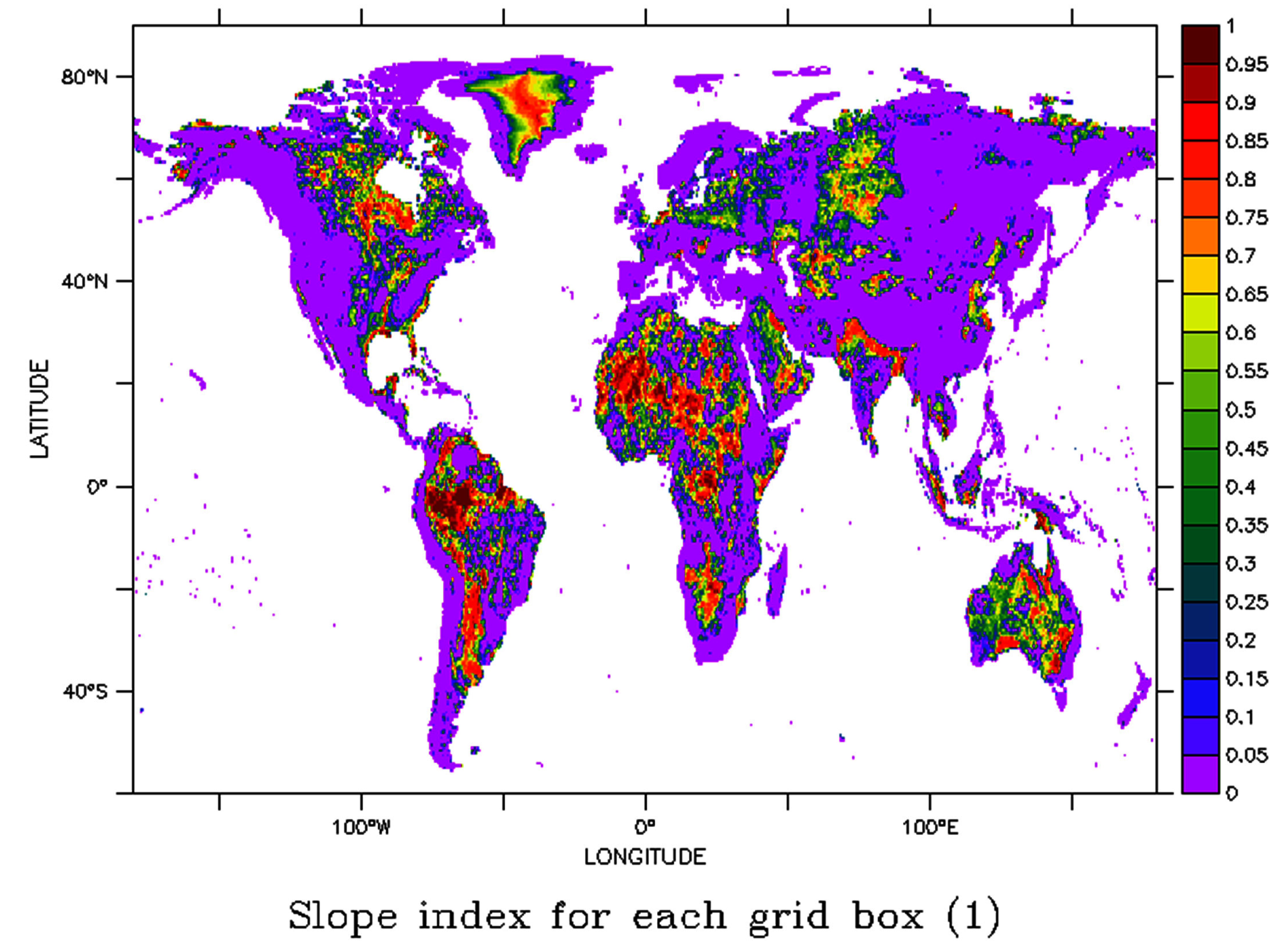
Figure 8:Map of the reinfiltration fraction produced by ORCHIDEE at the 0.5 resolution.
In practice, the fraction is defined in each grid-cell based on , the weighted area mean of the high-resolution slope, and a threshold slope (with a default value of 0.5%), such that local reinfiltration fraction decreases from 1 when , to 0 when :
Surface runoff is then reduced by the fraction , which is temporarily stored in the variable water2infilt, kept to be infiltrated at the following time step with the following throughfall, snowmelt, and return flows from the routing scheme if any. The variable water2infilt thus conveys memory of water storage, and belongs to the prognostic variables. Note, however, that it is integrated to the total soil moisture variables tmc and humtot (sections %s and %s)
The parameter is externalized and may be changed to modify the effectiveness of ponding. *** Cite Figure 8
1.7.3WIP: Soil water diffusion and drainage
1.7.4WIP: Compensation of numerical errors
1.7.5WIP: Soil hydraulic properties
1.7.6WIP: Soil water redistribution during land cover change
1.7.7WIP: Soil moisture nudging and forcing
Total runoff
Eventually, the two runoff terms in ORCHIDEE are a surface runoff (Hortonian runoff minus reinfiltration), and drainage, gravitational by default, at the bottom of soil column. The input water flux feeding infiltration () is the sum of throughfall and snowmelt during the time step, plus reinfiltration from the previous time step, and return flows from the routing scheme (from the flood plains and irrigation, see section ***), also from the previous time step.
For numerical convenience, infiltration proceeds before soil water redistribution, and bare soil evaporation (, see next section) is subtracted from the input water flux. If the former exceeds the latter, there is no infiltration, and the top boundary condition to water redistribution is a water demand amounting .
Note that the runoff terms can be modified during the time step to correct the cases of "oversaturation" (), which may arise from numerical errors when approaches saturation. If the drainage coefficient , or if soil freezing is allowed, all moisture above saturation is sent to surface runoff. Else, this "excess" moisture is sent to drainage.
*** provide an estimate of this error (mean and std, based on REF with PGF for IGEM, or Salma, or LS3MIP)
We assume unsaturated, 1D vertical, no lateral exchange *** Unless otherwise mentioned, the following text uses SI units. For instance, water flux variables are in kg m s.
A physically-based description of unsaturated soil water flow was introduced in ORCHIDEE by rosnay2002impact. It relies on a one-dimensional Richards equation, combining the mass and momentum conservation equations, but it takes the form of a Fokker-Planck equation, since the state variable is expressed as volumetric water content (m.m) rather than pressure head.
Due to the large scale at which ORCHIDEE is usually applied, we neglect the lateral fluxes between adjacent grid cells. *** Applied in each soil column and not grid-cell *** We also assume all variables to be horizontally homogeneous, so that the mass conservation equation relating the vertical distribution of to its flux field (m s) is:
In this equation, is depth below the soil surface, and is time (in m and s respectively). The sink term (m.m s) is due to transpiration and depends on the vertical profile of roots.
The flux field comes from the equation of motion known as darcy1856fontaines equation in the saturated zone, and extended to unsaturated conditions by buckingham1907studies:
and are the hydraulic conductivity and diffusivity (in m s and m s respectively). The latter defines the link between the volumetric soil moisture and the matric potential (in m):
The approach above was solved by making use of a finite difference integration. The Fokker-Planck equation defined by the combination of Eqs. 207-208 is solved using a finite difference method. To this end, the soil column is discretized using N nodes, defined by an index increasing from top to bottom, and where we calculate the values of (Figure 9). The middle of each consecutive couple of nodes represents the limit between two soil layers, except for the upper and the lower layers, for which the top/bottom interfaces are defined by the first/last nodes respectively. As a consequence, each soil layer holds only one node , and we define layer as the layer holding node . We can thus define the thickness of each layer by:
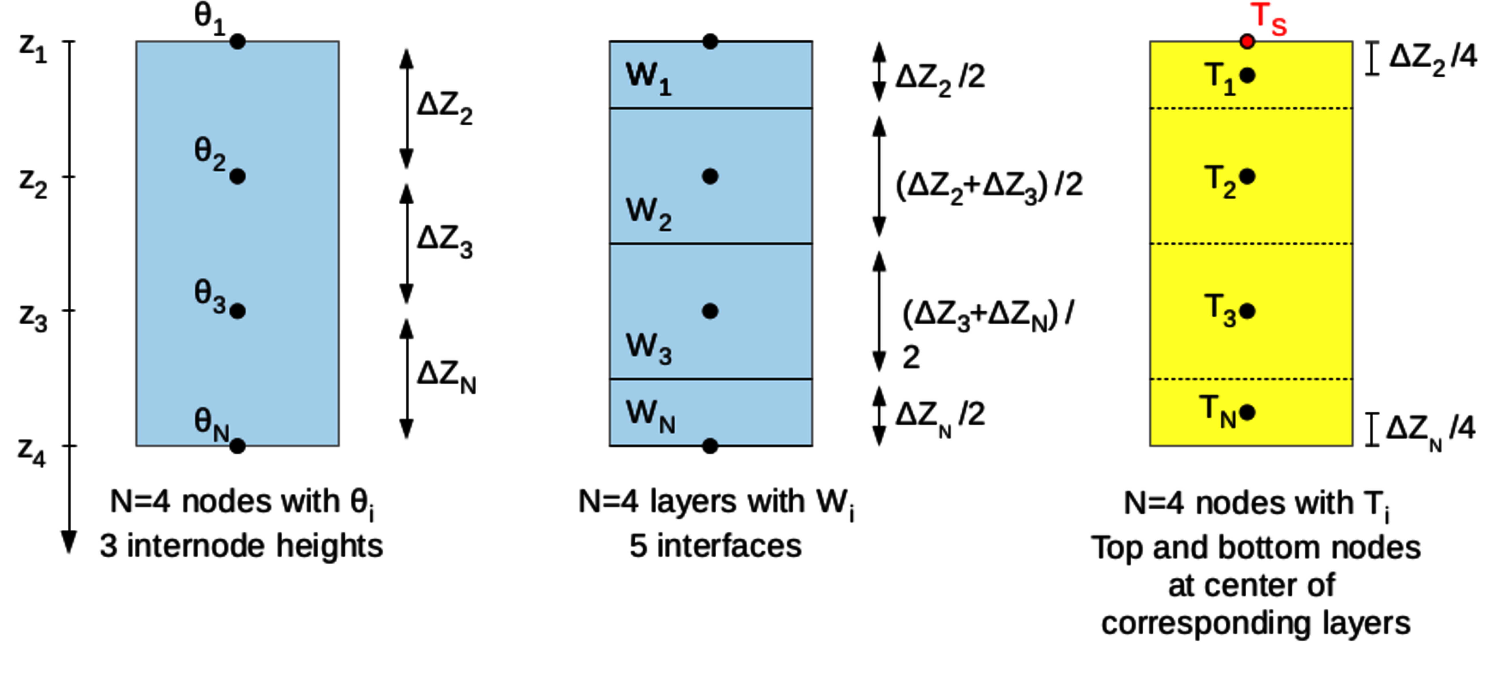
Figure 9:Illustration of soil vertical discretization, in case of 4 soil nodes and soils layers: for soil hydrology in blue on the left, with links between node positions, their local volumetric water content , the soil layers, their depth and integrated soil moisture , in the simple case of four equidistant nodes. Link with code’s names in Table %s. The correspondence with the nodes for the soil thermics appears on the yellow column to the right.
In these expressions, is the distance between nodes and , which have volumetric water contents and (Figure 9).
The total water content of each layer , (m), is obtained by integration of , assumed to undergo linear variations between two consecutive nodes:
Equation 207 can then be integrated between the nodes and over the time step , over which is assumed to be constantly equal to its value at (implicit scheme). This allows defining the water budget of each layer :
where is the integrated sink term and the water flux at the interface between layers and (both in m s).
The above flux is deduced from Equation 208, by approximating by the rate of increase between the equidistant neighbouring nodes and , and this leads to:
To get this expression, we also approximate the values of and at the layers’ interfaces by the arithmetic average of their values at the neighbouring nodes.
To make Equation 213 linear with respect to such as to construct a tridiagonal matrix system to solve , we discretize the interval in 50 regular subdomains where and are described by piecewise functions, respectively linear in and constant (Appendix %s).
Additional information is required to solve and .
It consists of water fluxes and at the top and bottom of the soil column respectively. These fluxes need to be prescribed as boundary conditions at each time step, and thus drive the evolution of the soil moisture profile (section %s).
By default, the bottom boundary condition to water flow in the soil is defined by free gravitational drainage:
But two other options are possible. The first one, originally proposed by deRosnay1999representation, consists in reducing the free drainage calculation by a coefficient :
where . This condition is equivalent to reducing the hydraulic conductivity under the bottom of the soil column, which could be achieved alternatively by enhancing the exponential decay of with depth. Setting makes the bottom totally impermeable as in the two-layer soil hydrology scheme of ORCHIDEE.
The second new boundary condition, proposed since Campoy2013phd, is to impose saturation under the calculation node chosen by the user:
This implies the presence of a water table inside the modeled soil column. To do so, we first solve the diffusion equation over the 2-m soil column assuming that , then we adjust the resulting soil moisture to bring it back to saturation at nodes and below, if either upward diffusion or root absorption made it drop to unsaturated values. The required water flux is assumed to enter the soil column through the soil bottom interface, and thus represents negative drainage. *** violation of water conservation, mention also the new scheme GWF
Van Genuchten relationships for hydraulic conductivity and diffusivity
The hydraulic parameters required by the diffusion equation solved in ORCHIDEE-2.0 (this document should refer to ORC4) are the hydraulic conductivity and diffusivity, and , which depend on volumetric water content . These relationships are given in ORCHIDEE-2.0 by the mualem1976new - van1980closed model:
which also writes:
There, is the saturated hydraulic conductivity (m s), (m) corresponds to the inverse of the air entry suction, and is a dimensionless parameter, related to the classical Van Genuchten parameter by:
The last Van Genuchten relationship defines the link between the matric potential (m), involved in the hydraulic diffusivity (Eq. 209), and the volumetric water content :
These equations, illustrated in Figure 10, assume that varies between the residual water content and the saturated water content , which leads to define relative humidity as . The hydraulic conductivity decreases with soil moisture, and this effect dominates the variations induced by soil texture (section %s). In contrast, the matrix potential , which corresponds to the retention forces by the unsaturated soil and is therefore negative, is stronger for weak soil moisture, at which it can efficiently counteract the gravitational forces controlled by . Diffusivity results from both influences and decreases with soil moisture like , but over a much smaller range owing to the counter influence of .
[This was moved from somewhere else and still needs to be integrated – FK] Soil hydraulic properties for the USDA classes are determined using the pedotransfer function of Carsel & Parrish (1988). The hydraulic properties of oxisoils were obtained by averaging the values found in literature, resulting in saturated hydraulic conductivity much higher than that of regular clay and closer to that of sand Tafasca, 2021.
![Van Genuchten relationship K(\theta), D(\theta), and \psi(\theta), for \theta in [\theta_r, \theta_s], based on Eqs. %s, %s, and %s, for the 12 USDA texture classes *** a link must be made with texture and PTFs cf. section %s. The three thick lines show the three texture classes used with the simplified Zobler map (Table %s). The difference between the first two panels is that the second one uses a logarithmic axis for K(\theta).](/build/VG12-fe1f1ff19b0b25564f8cdd405d783f1d.webp)
Figure 10:Van Genuchten relationship , , and , for in , based on Eqs. 217, 219, and 221, for the 12 USDA texture classes *** a link must be made with texture and PTFs cf. section %s. The three thick lines show the three texture classes used with the simplified Zobler map (Table %s). The difference between the first two panels is that the second one uses a logarithmic axis for .
Hydraulic conductivity decrease with depth due to compaction
Following dorgeval2006thesis and dOrgeval2008sensitivity, several modifications of , thus , with depth are implemented in ORCHIDEE-2.0. Firstly, as suggested by beve:79, is assumed to decrease exponentially with depth (below the top 30 centimeters with the default parameters) to represent the effect of compaction:
Here, is the depth below the soil surface, is the reference value of based on soil texture (section 1.7). The other three parameters are constants, which are independent from the PFT, the soil column, and the soil texture: is the depth at which the decrease of starts; is the decay factor (in m); and cannot be smaller than . The default values are m, m, and , so that is identical for all nodes below 1.45 m, and equal in this case to 0.1 .
Hydraulic conductivity increase towards the surface due to bioturbation
An increase of towards the soil surface is also taken into account, because the presence of vegetation tends to increase the soil porosity in the root zone and therefore to increase infiltration capacity beve:82beve:84. This effect is tightly linked to the decrease of with depth, and could seem redundant, but it is described independently to introduce a dependency on the root density profile. Root density is assumed to decrease exponentially with depth, as defined by a root decay factor (in m), which is a PFT characteristic (ranging from 0.4 m in tropical forests to 4 m in C3 cropland):
For each MC with vegetation (thus excluding the bare soil MC), a multiplicative factor is defined as a function of depth and :
is a constant taken as the maximum given by carsel1988developing for the sandy texture, so = 7128.0 mm.d. As shown by Figure 11, this formula leads to increase the saturated conductivity exponentially for (which ranges between 0.25 m for grasses and crops, to 1.25 m for forests, when using the defaults values of for the multi-layer hydrology. It can be noted that the maximum , at the surface, is independent from and the vegetation type, and is always .
The resulting saturated conductivity for the soil column is eventually given by the following expressions:
where is given by Eq. 222, and is the fraction of MCs belonging to the soil column .
The above equations assume that is not modified by roots in the bare soil PFT (), and were first been introduced by dOrgeval2008sensitivity to obtain a reasonable evapotranspiration variability in Hapex-Sahel simulations. This work used instead of , leading to variable over time, since . It was changed to make constant if the PFT does not change.
Combined effects on hydraulic conductivity and other parameters
Eventually, the vertical profile of the effective saturated hydraulic conductivity is given in each soil column by:
The effect of each factor and is illustrated in Figure 11. In practice, these two factors are used to define: (i) the non-saturated hydraulic conductivity and diffusivity (as detailed in appendix %s) required for water redistribution based on the Richards equation; (ii) the saturated and non-saturated hydraulic conductivity to calculate infiltration (section 1.7.2). The non-saturated parameters also depend on the Van Genuchten parameters and , which are modified according to as explained in below.

Figure 11:Profiles of saturated hydraulic conductivity for a sandy loam soil. The final profiles are in orange for a grass PFT, and in yellow for a forest PFT. *** MUST BE CORRECRED TO GET A CONSTANT KS between 1.5m and 2m equal to /10=106mm/day ***
To introduce a consistency between and the parameters and , the latter can also be calculated, based on their log-log regression with , using the values given by carsel1988developing for the 12 USDA soil textures. The resulting regressions appear in Fig 4.14 of dorgeval2006thesis, and are defined by:
where = 0.95, = 0.34, = 0.12 m, and = 0.53. The parameters and equal 42 and 2500 respectively, but they vanish when combining equations.
Given the texture, we know , and (Eqs. 222 and 223). From Eqs. 229 and %s, it comes:
In ORCHIDEE-2.0, these relationships are used to define changes in and resulting from the decrease of with depth below 30 cm (section ??), but they are not used to change and as a result of increase with roots (section ??).
Link to soil texture maps
Soil texture and related parameters are assumed to be horizontally uniform within each grid-cell. At the beginning of each simulation, a pre-processing step allows to extract the domimant soil texture (i.e the texture class occupying the largest fractional area of the grid-cell) given the resolution of the simulation and the chosen input soil map.
As detailed in sections %s and %s, most soil properties are inferred from this dominant soil texture. It is not the case, however, for the clay fraction, used in the STOMATE module for soil carbon calculations, and defined as the weighted-area average of the clay percent of each texture class inside a grid-cell. The mean percent of sand and silt particles is computed similarly for output. *** is percent sand used for thermal properties ?
In this framework, ORCHIDEE-2.0 accounts for the soil’s characteristics owing to the Van Genuchten parameters (, , , and ), as well as secondary parameters derived from the latter ones (section %s). *** Clay fraction for STOMATE and:
*** To this end, we use the look-up tables provided by carsel1988developing to define one single central value for each class and parameters, which corresponds to the simplest pedotransfer function vanlooy2017pedotransfer. *** Clay fraction is defined by the mean granumometric composition for each USDA class, as defined in carsel1988developing.
The field capacity and wilting point are important threshold soil moistures, which control available water capacity, and are related to soil moisture stresses (section %s). The corresponding volumetric water contents, further noted and , can be related to and (Van Genuchten relationships), by means of characteristic soil matric potentials. These parameters are derived using the Van Genuchten relationships, based on a soil matric potential of -3.3 m (-1 m for sandy soils following richards1944moisture) for , and -150 m (permanent wilting point) for , so they vary with soil texture.
The resulting values of and are given in Table 3, with all the main properties of the 12 USDA soil textures, including the values of (if not modified to follow ) and (Appendix %s). Figure 12 further shows the spatial distribution of wilting point and field capacity based on the texture map of Reynolds et al. (2000) and an horizontal resolution of 144 143, used in many IPSL simulations for CMIP-6. *** Add AWC*** Attention, le calcul est faux si on n’a pas alpha constant *** mettre les cartes pour Zobler et Reynolds
Table 3:Values of important soil parameters for the 12 USDA texture classes. *** AWC(2m) gives the available water capacity of a 2m soil, calculated in mm as AWC(2m) = 2000 . The values of and are calculated assuming vertically uniform and (the very fine textures, for classes 11 and 12, lead to problematic values at very low soil moistures *** replace with code + units of d2 and d50 are not good values
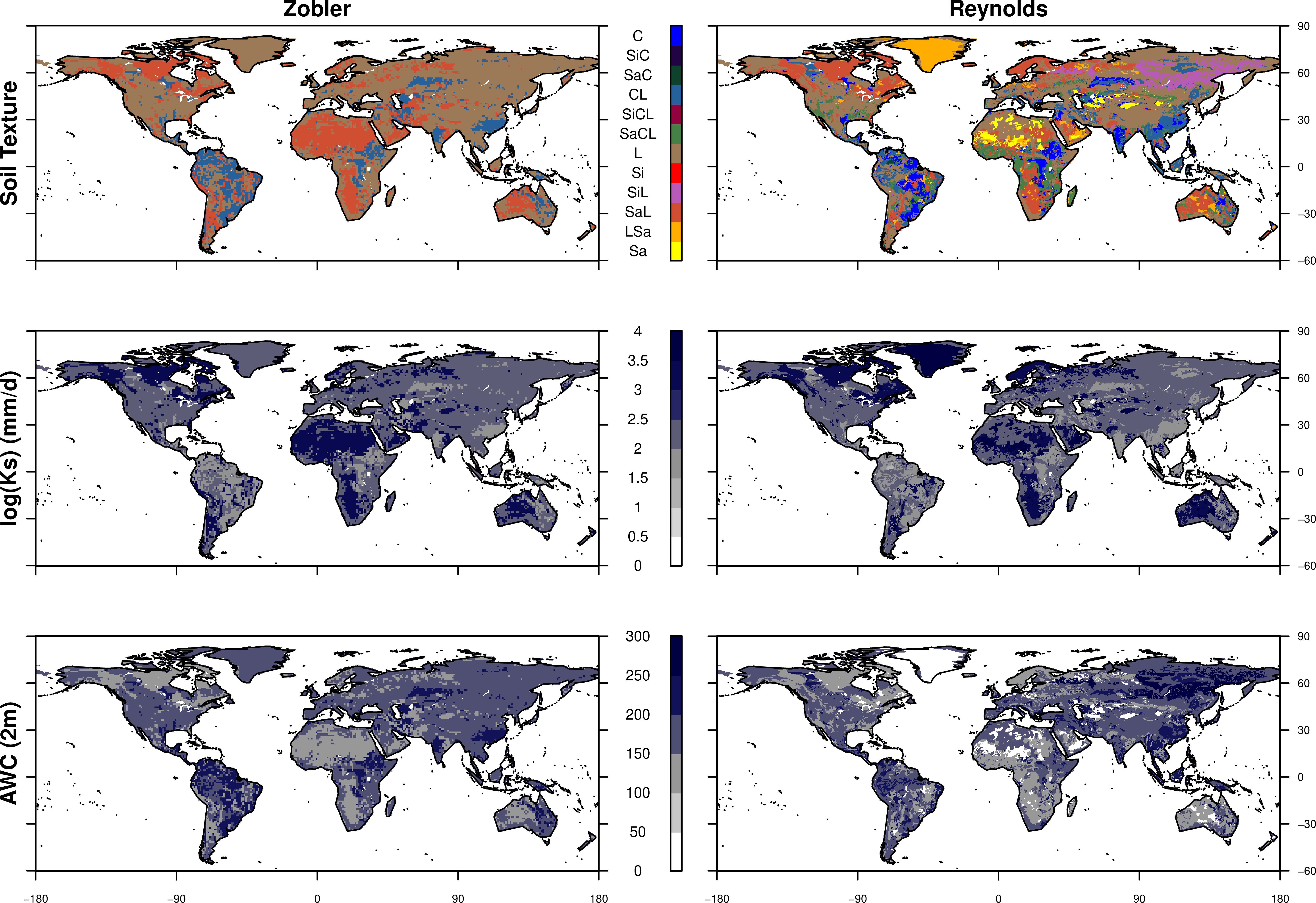
Figure 12:The two soil texture maps available in ORCHIDEE-2.0 (top row), with important derived hydrologic properties: saturated hydraulic conductivity (values in mm.d tranformed with ) (middle row), and available water content AWC (in mm) over the 2m-soil depth (bottom row). All the maps are produced at the 0.5° resolution, based on the dominant soil texture at this resolution. *** Zobler modified
.
*** Since we solve one independent water budget per soil column, the number of times the diffusion scheme is used per grid-cell is defined by the number of soil columns.
Soil moisture can be quantified by different variables in ORCHIDEE (see Table %s for notations):
the volumetric water contents , which give the local moisture at the calculation nodes, in m.m (Figure 9),
the total water contents of the soil layers defined in Figure 9, and calculated using Eqs 211-%s, in kg.m or mm,
the total water content of the soil column: , in kg.m or mm. It is equivalent to the vertical integration of .
the total water content of litter, defined in ORCHIDEE as the four top soil layers: , in kg.m or mm.
All these variables are different in the different soil columns of one ORCHIDEE grid-cell, and we can define two types of spatial averages across the soil columns. In the following, we will indicate the simple weighted average across the different soil columns by an overbar: , for the mean total soil moisture for instance. This value gives an average in kg per m of , and the conversion to kg per m of defines .
Finally, all these variables can be defined for total, liquid, and solid water, the latter two being identified by the exponents and in this document.
1.8Routing to the oceans
Eventually, the two runoff terms in ORCHIDEE are a surface runoff (Hortonian runoff minus reinfiltration), and drainage, gravitational by default, at the bottom of soil column. The input water flux feeding infiltration () is the sum of through-fall and snowmelt during the time step, plus reinfiltration from the previous time step, and return flows from the routing scheme (from the flood plains and irrigation, see USE dynamic link: section 7.3), also from the previous time step. For numerical convenience, infiltration proceeds before soil water redistribution, and bare soil evaporation () is subtracted from the input water flux. If the former exceeds the latter, there is no infiltration, and top boundary condition to water redistribution is a water demand amounting .
The routing scheme calculates the lateral water flow through river networks across the continent into the ocean. The routing scheme of ORCHIDEE (Polcher (2003)) was described in Ngo-Duc et al. (2007), d'Orgeval et al. (2008) and Guimberteau et al. (2014). It is based on a large-scale cell-to-cell methodology in which the watershed is represented as a single grid cell or a network of equal grid cells (Singh, 1989). Each of the interconnected grid cell is approximated as a cascade of linear reservoirs which do not interact with the atmosphere. When activated in ORCHIDEE, the routing scheme transforms every day ( = 86400 s) the runoff simulated by SECHIBA into river discharge and computes an hydrograph at any grid cell and not only at the outlet. The routing scheme is based on a parametrization of the water flow on a global scale (Miller et al., 1994; Hagemann and Dumenil, 1998). The global map of 6930 watersheds (Oki et al. (1999); Fekete et al. (1999); Vörösmarty et al. (2000)) delineates the boundaries of the basins. By default, only the 50 largest basins are selected in the model ( = 50). This map provides also single water flow direction among the 11 possibilities within each grid cell: 8 directions towards another grid cell (N, NE, E, SE, S, SW, W, NW), one direction towards the endorheic lakes, one direction towards the ocean and one direction accounting for the water from small rivers which flows in a disperse way into the ocean. The resolution of the basin map is 0.5°, coarser than usual resolution used when land surface models are applied. Therefore, we can have more than one basin in SECHIBA grid cell (sub-basins) and the water can flow either to the next sub-basin within the same grid cell or to the neighboring cell. No more than 7 sub-basins can be included in a grid cell ( = 7). For a selected basin, cell-to-cell flow through the system of digital river networks is modelled using the continuity equation computed for each reservoir:
where (kg) is the water amount in the reservoir considered ( = 1, 2 or 3) and and (both in kg/day) are respectively the total inflow and outflow of the reservoir .
In each sub-basin, runoff simulated by SECHIBA is transformed into river discharge emanating from the so-called fast and slow reservoirs, designed to account for the delay and attenuation of overland flow and groundwater flow, respectively, at the grid-cell scale. The slow reservoir ( = 3) collects the drainage (in kg/day), whereas the fast reservoir ( = 2) collects the surface runoff (in kg/day). Outflow from these two reservoirs becomes streamflow at the outlet of the sub-basin, and feeds the stream reservoir ( = 1) of the next downstream sub-basin, which also receives inflow from all upstream stream reservoirs:
The outflow of the reservoir is assumed to be related to the stored volume of water by a linear relationship:
Travel time within the reservoir depends on a characteristic timescale (day), which is the product of a topographical water retention index (in km) and a time constant (in day/km):
does not vary horizontally but distinguishes the three reservoirs, while characterizes the impact of topography on travel time in each sub-basin, and is assumed to be the same in the three reservoirs of a given grid cell, even though it derives from stream-routing principles introduced by Ducharne et al. (2003):
This travel time is thus assumed to be proportional to stream length (in m) in the sub-basin, and inversely proportional to the square root of stream slope (). The lengths and slopes are computed at the 0.5° × 0.5° resolution from the topographical map of Vörösmarty et al. (2000a, 2000b). This can be seen as a simplification of the Manning formula (Manning (1895)), where the time constant compensates for the missing terms. The values of the time constants, , were initially calibrated over the Senegal Basin then generalized for all the basins of the world (Ngo-Duc et al. (2007)). The stream reservoir has the lowest constant ( = 0.24 10 day/km). value has been set to = 3.0 10 day/km and = 25.0 10 day/km in the fast and slow reservoirs respectively.
- Milly, P. C. D. (1992). Potential Evaporation and Soil Moisture in General Circulation Models. J. Climate, 5, 209–226. 10.1175/1520-0442
- de Rosnay, P. (2002). Impact of a physically based soil water flow and soil-plant interaction representation for modeling large-scale land surface processes. Journal of Geophysical Research, 107(D11), 4118. 10.1029/2001JD000634
- Campoy, A., Ducharne, A., chëruy, F., Hourdin, F., Polcher, J., & Dupont, J. (2013). Response of land surface fluxes and precipitation to different soil bottom hydrological conditions in a general circulation model. Journal of Geophysical Research: Atmospheres, 118(19), 10–725.
- Damour, G., Simonneau, T., Cochard, H., & Urban, L. (2010). An overview of models of stomatal conductance at the leaf level. In Plant, Cell and Environment (Vol. 33). 10.1111/j.1365-3040.2010.02181.x
- Mencuccini, M., Manzoni, S., & Christoffersen, B. (2019). Modelling water fluxes in plants: from tissues to biosphere. In New Phytologist (Vol. 222). 10.1111/nph.15681
- Fatichi, S., Pappas, C., & Ivanov, V. Y. (2016). Modeling plant–water interactions: an ecohydrological overview from the cell to the global scale. In Wiley Interdisciplinary Reviews: Water (Vol. 3). 10.1002/wat2.1125
- Kennedy, D., Swenson, S., Oleson, K. W., Lawrence, D. M., Fisher, R., da Costa, A. C. L., & Gentine, P. (2019). Implementing Plant Hydraulics in the Community Land Model, Version 5. Journal of Advances in Modeling Earth Systems, 11(2). 10.1029/2018MS001500
- de Kauwe, M. G., Medlyn, B. E., Ukkola, A. M., Mu, M., Sabot, M. E. B., Pitman, A. J., Meir, P., Cernusak, L. A., Rifai, S. W., Choat, B., Tissue, D. T., Blackman, C. J., Li, X., Roderick, M., & Briggs, P. R. (2020). Identifying areas at risk of drought-induced tree mortality across South-Eastern Australia. Global Change Biology, 26(10). 10.1111/gcb.15215
- Yin, X., & Struik, P. C. (2009). C3 and C4 photosynthesis models: An overview from the perspective of crop modelling. NJAS - Wageningen Journal of Life Sciences, 57(1), 27–38. 10.1016/j.njas.2009.07.001
- Tuzet, A., Perrier, A., & Leuning, R. (2003). A coupled model of stomatal conductance, photosynthesis and transpiration. Plant, Cell and Environment, 26(7). 10.1046/j.1365-3040.2003.01035.x
- Tuzet, A., Granier, A., Betsch, P., Peiffer, M., & Perrier, A. (2017). Modelling hydraulic functioning of an adult beech stand under non-limiting soil water and severe drought condition. Ecological Modelling, 348. 10.1016/j.ecolmodel.2017.01.007
- Bonan, G. B., Williams, M., Fisher, R. A., & Oleson, K. W. (2014). Modeling stomatal conductance in the earth system: Linking leaf water-use efficiency and water transport along the soil-plant-atmosphere continuum. Geoscientific Model Development, 7(5), 2193–2222. 10.5194/gmd-7-2193-2014
- van Genuchten, M. (1980). A closed-form equation for predicting the hydraulic conductivity of unsaturated soils. Soil Science Society of America Journal, 44(5), 892–898.
- Campbell, G. S. (1986). Soil Physics with Basic. 1986. Soil Science, 142(6). 10.1097/00010694-198612000-00007
- Yang, J., Duursma, R. A., Kauwe, M. G. D., Kumarathunge, D., Jiang, M., Mahmud, K., Gimeno, T. E., Crous, K. Y., Ellsworth, D. S., Peters, J., Choat, B., Eamus, D., & Medlyn, B. E. (2019). Incorporating non-stomatal limitation improves the performance of leaf and canopy models at high vapour pressure deficit. Tree Physiology, 39(12). 10.1093/treephys/tpz103